Part A: IMAGE WARPING and MOSAICING
Overview
In the first part of Project 4, I started by capturing photos with a fixed center of projection and calculating the homography matrix using least squares to align the images. This enabled me to warp images toward a reference, perform image rectification, and blend them seamlessly into a mosaic using weighted averaging techniques.
Shoot the Pictures
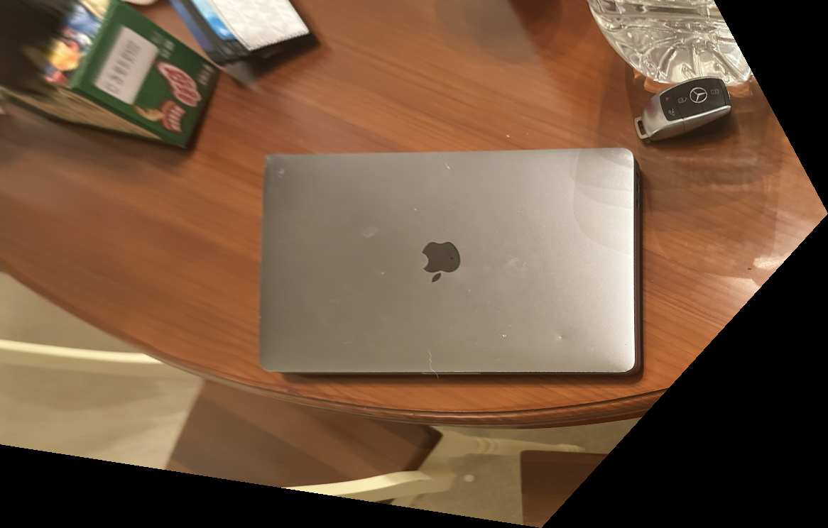
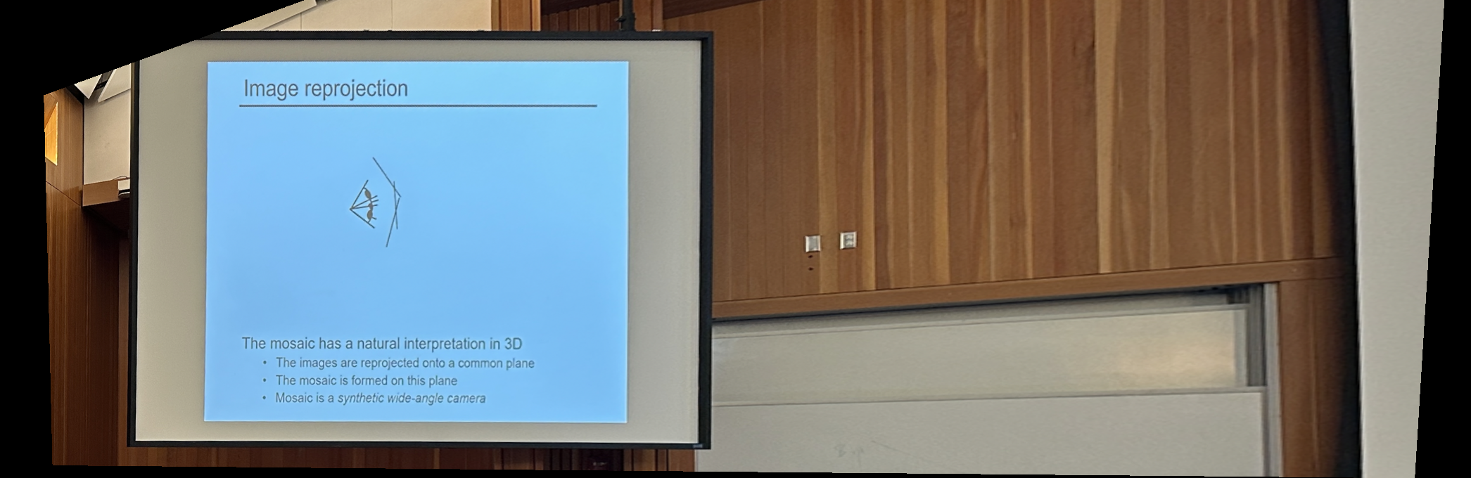
I took the following pictures for image rectification and blended them into a mosaic.
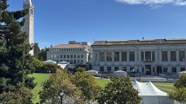
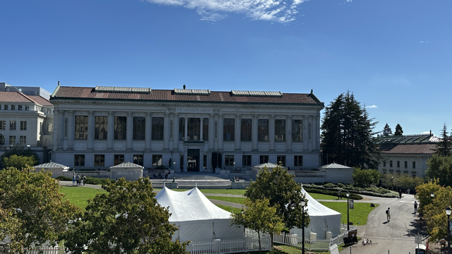
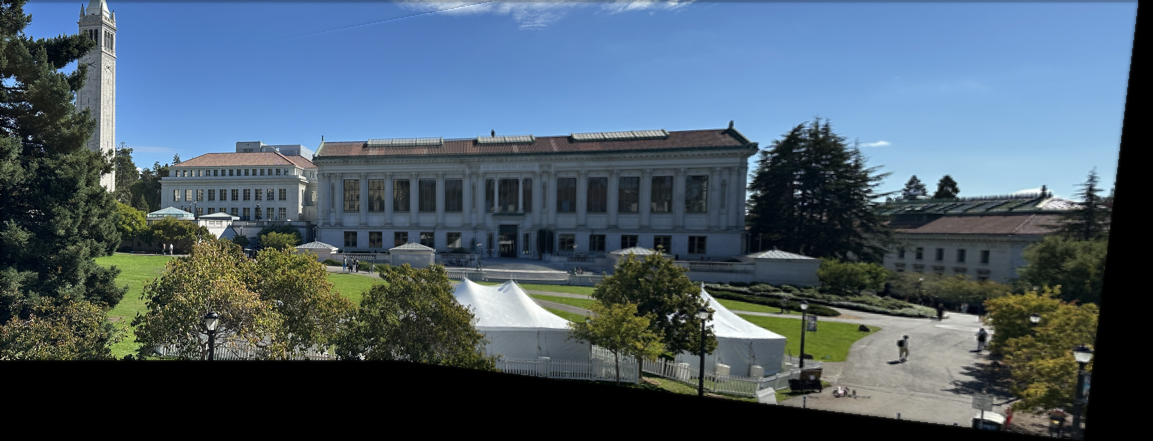
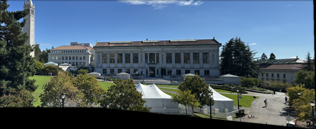
Library
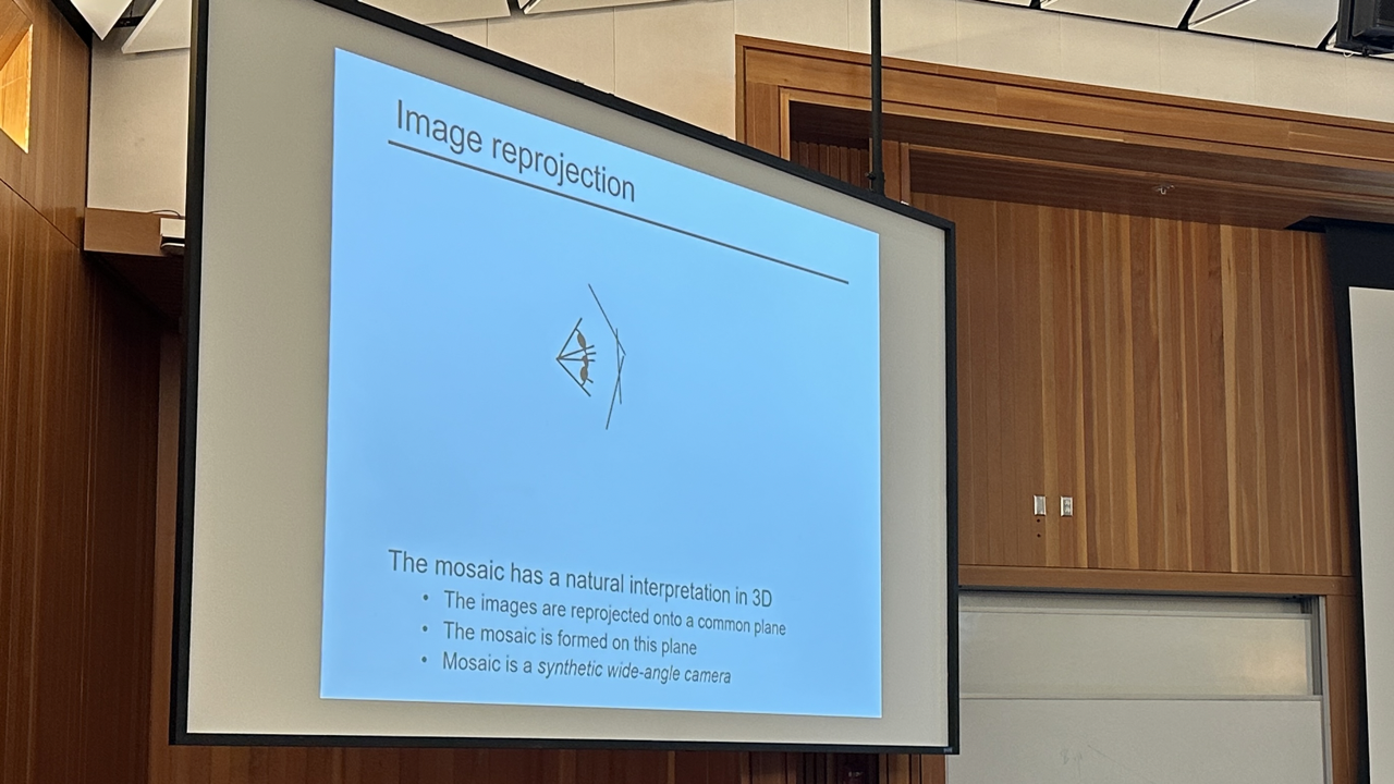
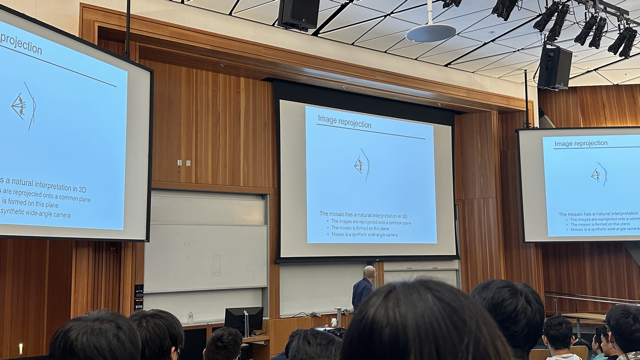
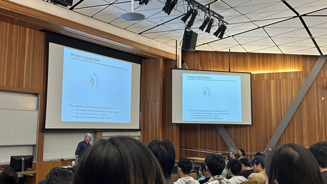
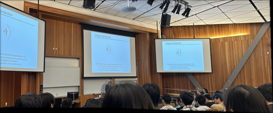
CS180 lecture
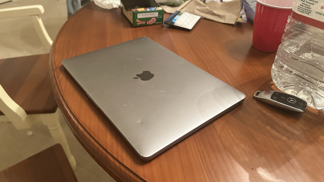
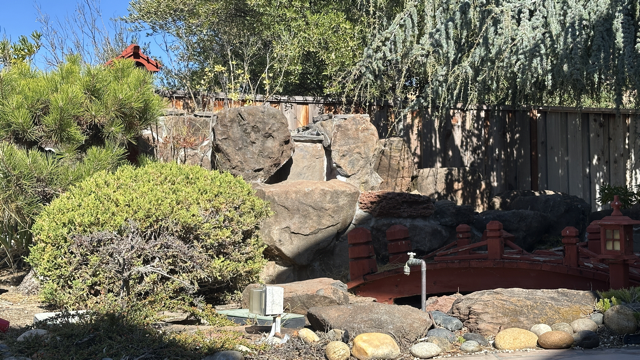
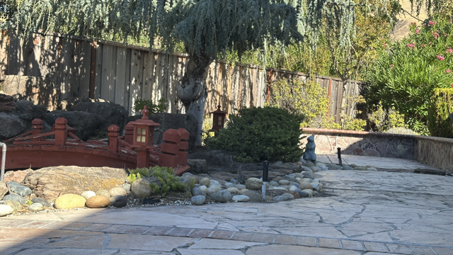
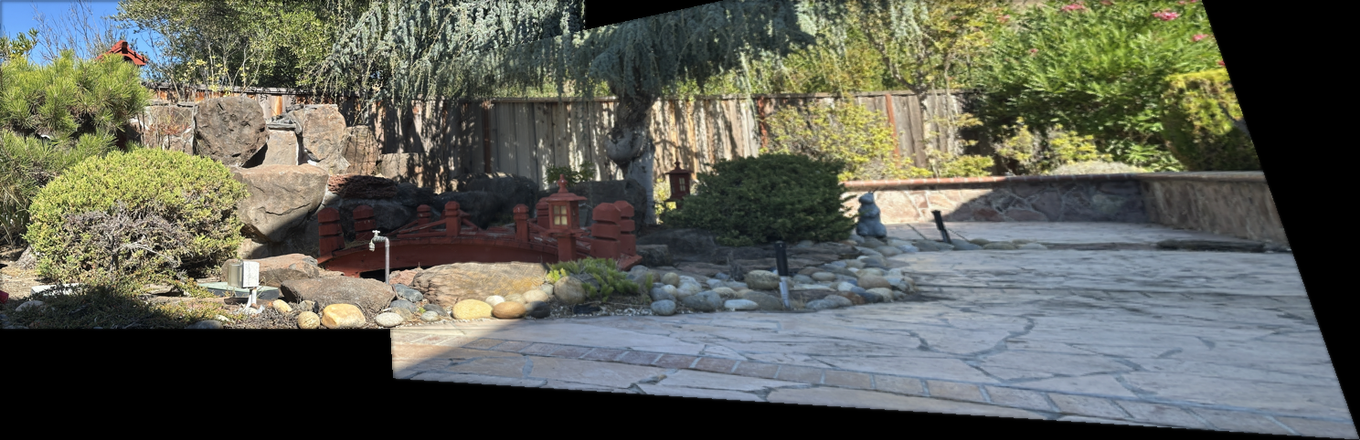
My garden
Recover Homographies
To align images, we need to recover the homography transformation, represented as \(p{\prime} = Hp\), where H is a 3x3 matrix with eight degrees of freedom. The function to compute this can be written as:
H = computeH(im1_pts, im2_pts)
H can be described as:
\[ H = \begin{bmatrix} h_1 & h_2 & h_3 \\ h_4 & h_5 & h_6 \\ h_7 & h_8 & 1 \\ \end{bmatrix} \]According to \(p{\prime} = Hp\)
\[ \begin{bmatrix} w p_1{\prime} \\ w p_2{\prime} \\ w \end{bmatrix} = \begin{bmatrix} h_1 & h_2 & h_3 \\ h_4 & h_5 & h_6 \\ h_7 & h_8 & 1 \end{bmatrix} \begin{bmatrix} p_1 \\ p_2 \\ 1 \end{bmatrix} \]After we expand the formulation above, we can get:
\[ \begin{cases} h_1 p_1 + h_2 p_2 + h_3 - h_7 p_1 p_1{\prime} - h_8 p_2 p_1{\prime} = p_1{\prime} \\ h_4 p_1 + h_5 p_2 + h_6 - h_7 p_1 p_2{\prime} - h_8 p_2 p_2{\prime} = p_2{\prime} \end{cases} \] \[ \begin{bmatrix} p_1 & p_2 & 1 & 0 & 0 & 0 & -p_1 p_1{\prime} & -p_2 p_1{\prime} \\ 0 & 0 & 0 & p_1 & p_2 & 1 & -p_1 p_2{\prime} & -p_2 p_2{\prime} \end{bmatrix} \begin{bmatrix} h_1 \\ h_2 \\ h_3 \\ h_4 \\ h_5 \\ h_6 \\ h_7 \\ h_8 \end{bmatrix} = \begin{bmatrix} p_1{\prime} \\ p_2{\prime} \end{bmatrix} \]Thus, if we have a seris of keypoints, we can compute homography by least squares
Warp the Images
I use inverse warping to align the images to their reference image. First, I compute the inverse of the homography matrix (H). Then, I map the canvas pixels back to the input image using the inverse of H. Finally, I use scipy.interpolate.griddata to interpolate the pixel values.
Image Rectification
In order to rectify image, I firstly pre-define four keypoints and then compute the homography. Finally, I warp the image to the canvas.
Blend the images into a mosaic
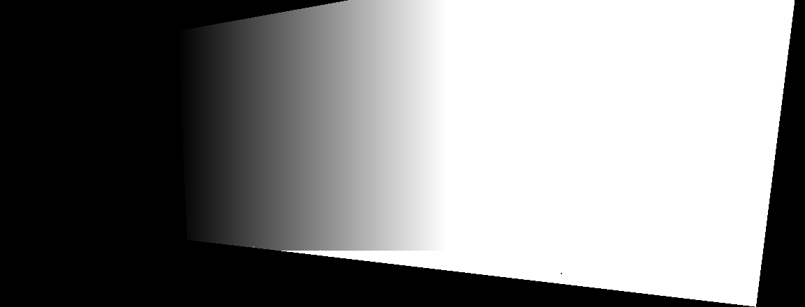
To create a mosaic, I select a reference image from the set and use inverse warping to align the other images to it. Next, I compute the maximum canvas size and apply distance transformation to create a mask. The alpha value is calculated as the ratio of the distance to the nearest non-overlapping pixel to the overlap length. To blend the images seamlessly, I use Laplacian Pyramid blending, as implemented in Project 2.
Library

CS180 classroom
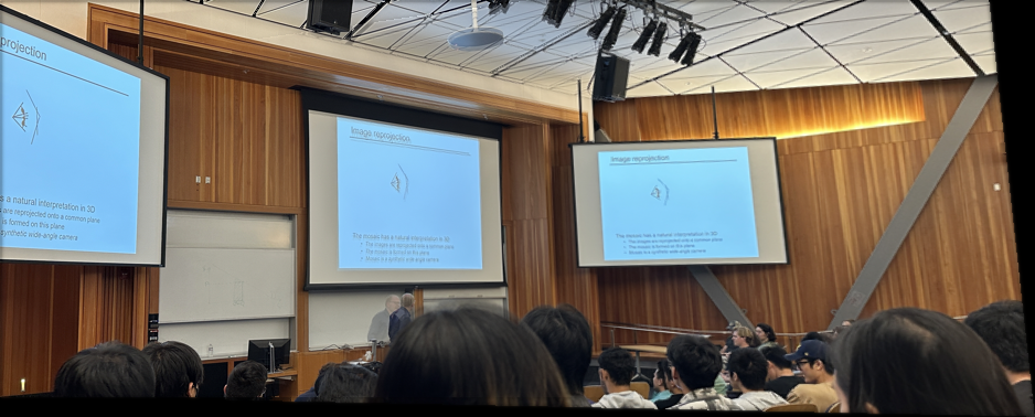
CS180 classroom

Part B: FEATURE MATCHING for AUTOSTITCHING
Overview
In this project, I aimed to automate image stitching into a mosaic while deepening my understanding of implementing research papers. Following the steps outlined in “Multi-Image Matching using Multi-Scale Oriented Patches” by Brown et al., I first detected corner features using the Harris Interest Point Detector and refined them through Adaptive Non-Maximal Suppression. I then extracted 8x8 feature descriptors from larger 40x40 windows, ensuring proper normalization for consistency. To match features between images, I applied Lowe’s method of thresholding the ratio between the first and second nearest neighbors, filtering out unreliable matches. Finally, I computed a robust homography using a 4-point RANSAC algorithm to accurately align the images.
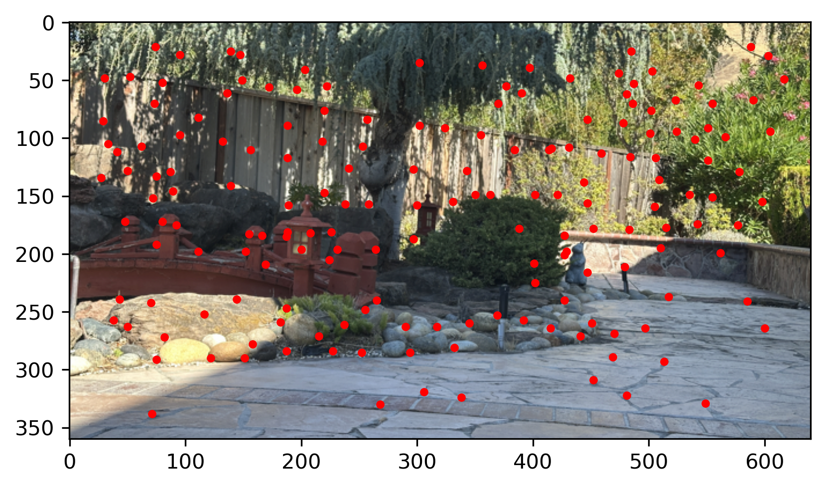
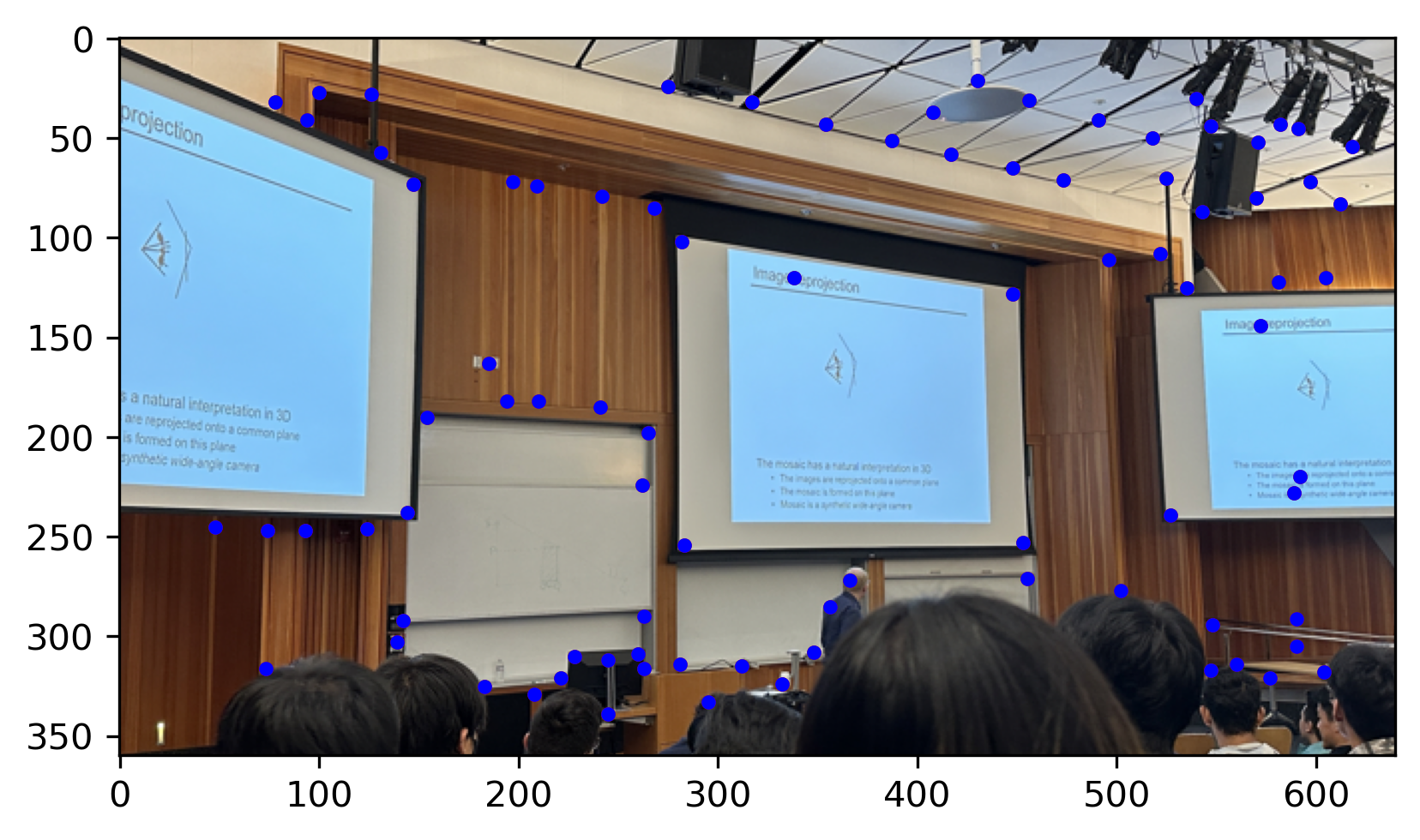
step1: Harris Interest Point
In corner dection, we use the Harris interest point detector.
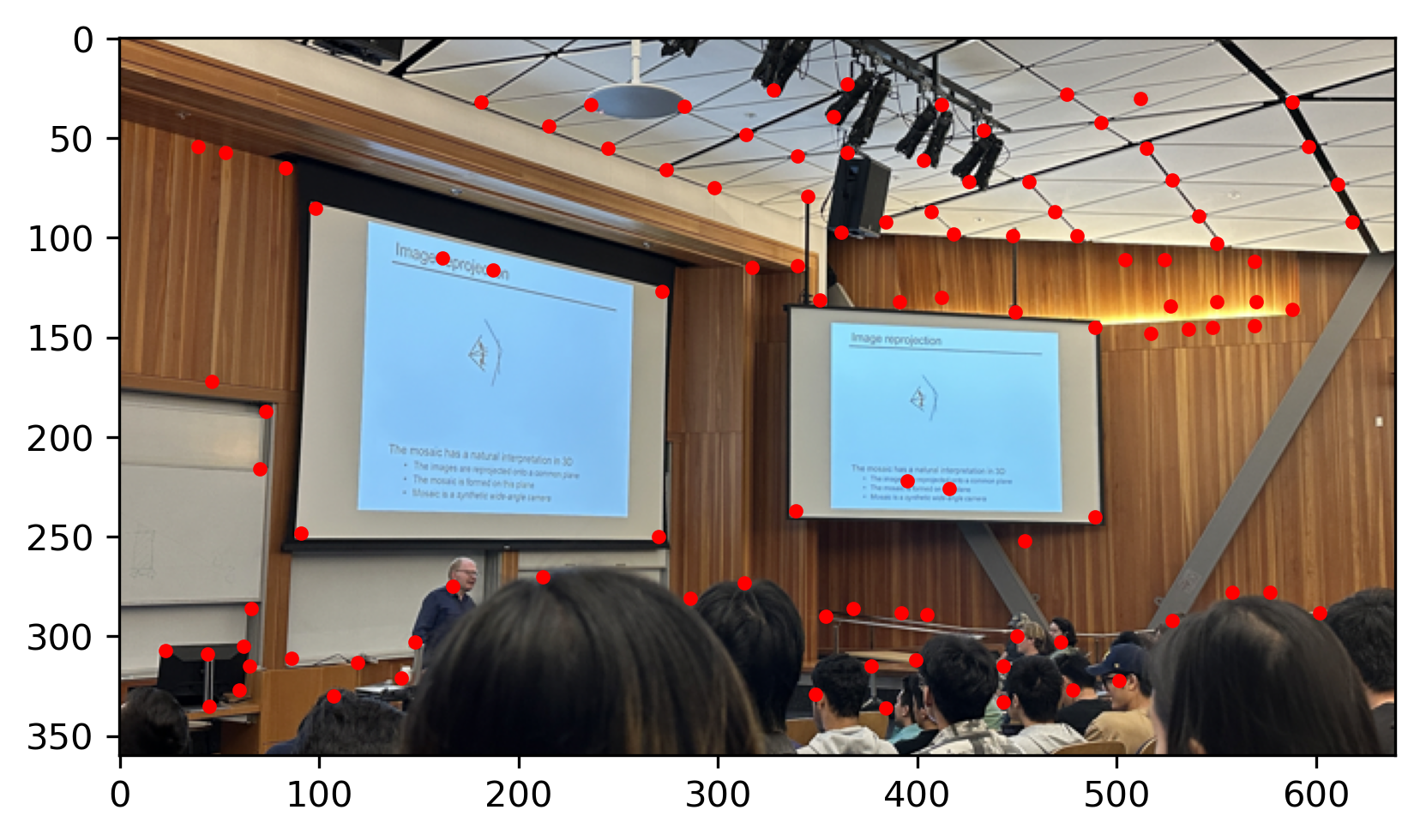
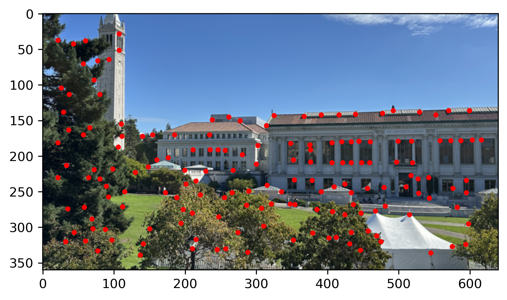
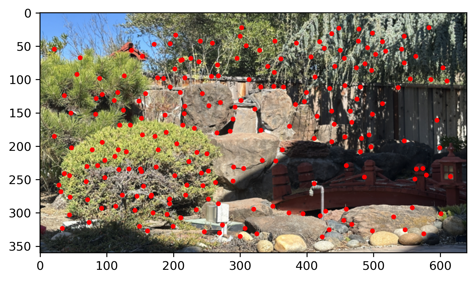
The examples below is the Harris Interest Point of the images:
CS180 lecture

Library
My garden
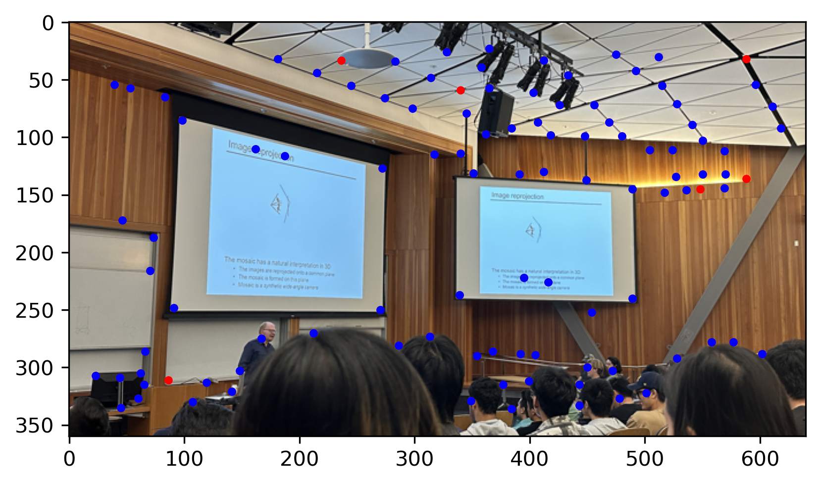
Step2: Adaptive Non-Maximal Suppression
Adaptive Non-Maximal Suppression (ANMS) selects the most prominent features by retaining only the points with the highest corner strength while ensuring they are sufficiently spaced apart. It suppresses weaker points within a certain radius around stronger features, enhancing feature distribution across the image.
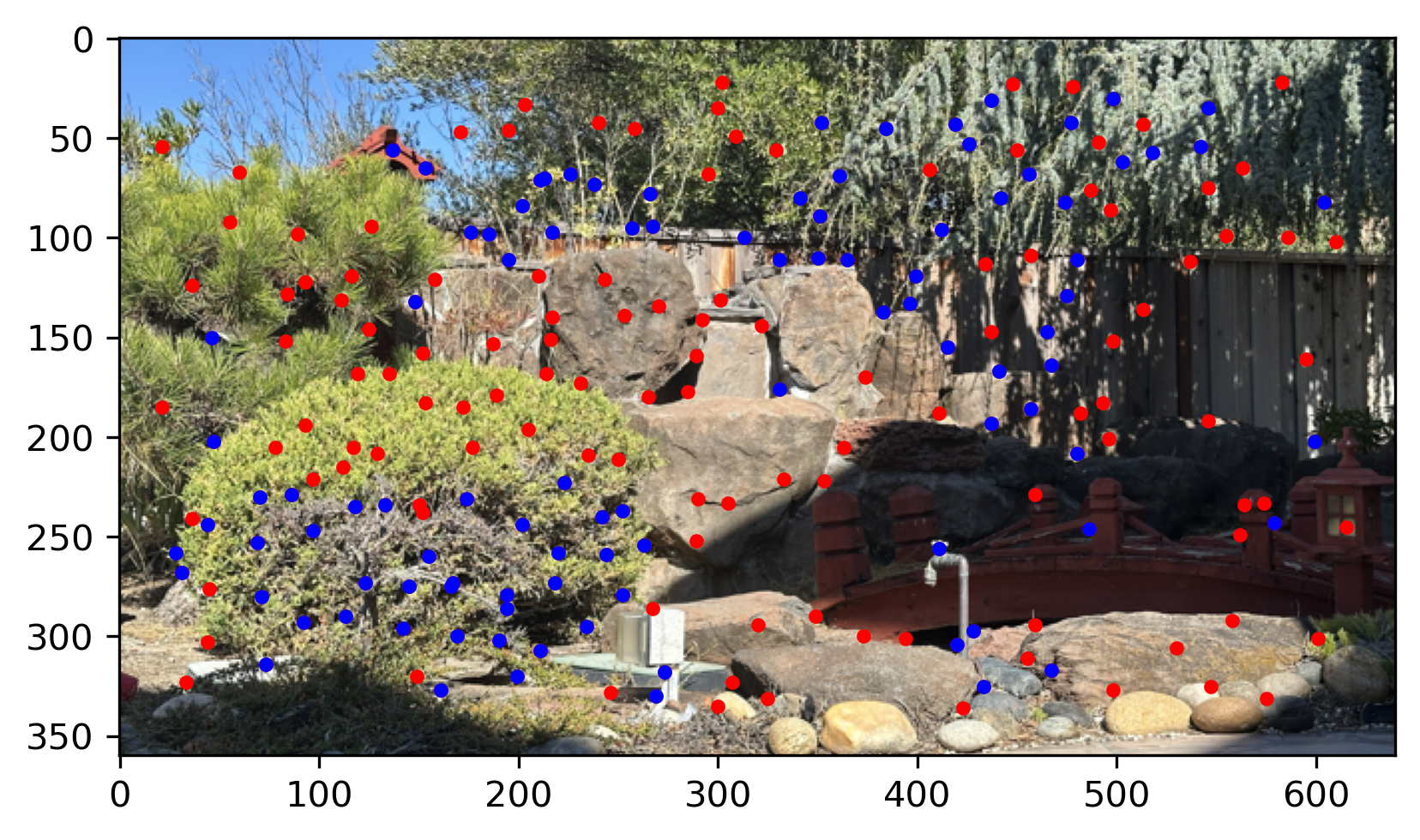
See the results of ANMS below. The red point is the Harris Interest Point and The blue point is the Harris Interest Point after ANMS
CS180 lecture
Library
My garden

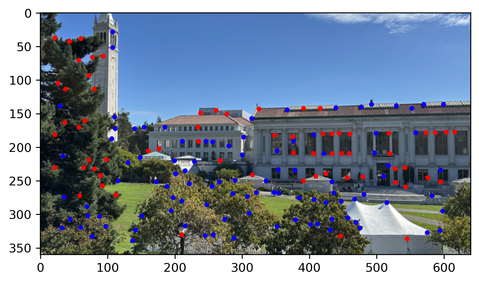
Step3: Feature Descriptor Extraction & Feature Matching
The feature extraction process begins by iterating through interest points, extracting a 40x40 pixel patch around each one if it fits within the image boundaries. The patch is then smoothed using a Gaussian filter to reduce noise and resized to an 8x8 patch with anti-aliasing. Next, bias/gain normalization is applied by subtracting the mean and dividing by the standard deviation. The resulting 8x8 patch is flattened into a vector and stored as a feature descriptor. Finally, all descriptors are collected and returned as an array.
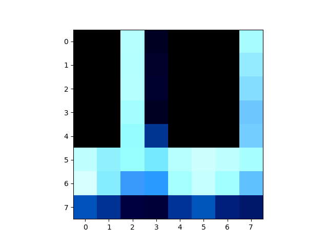
There is one descriptor of an image show below:
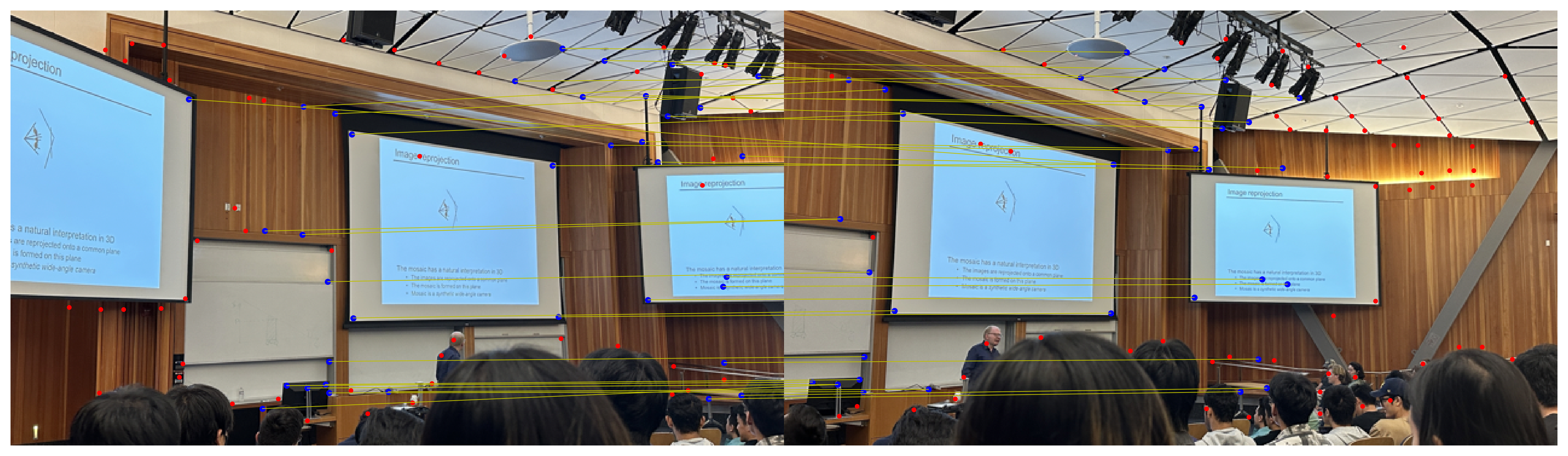
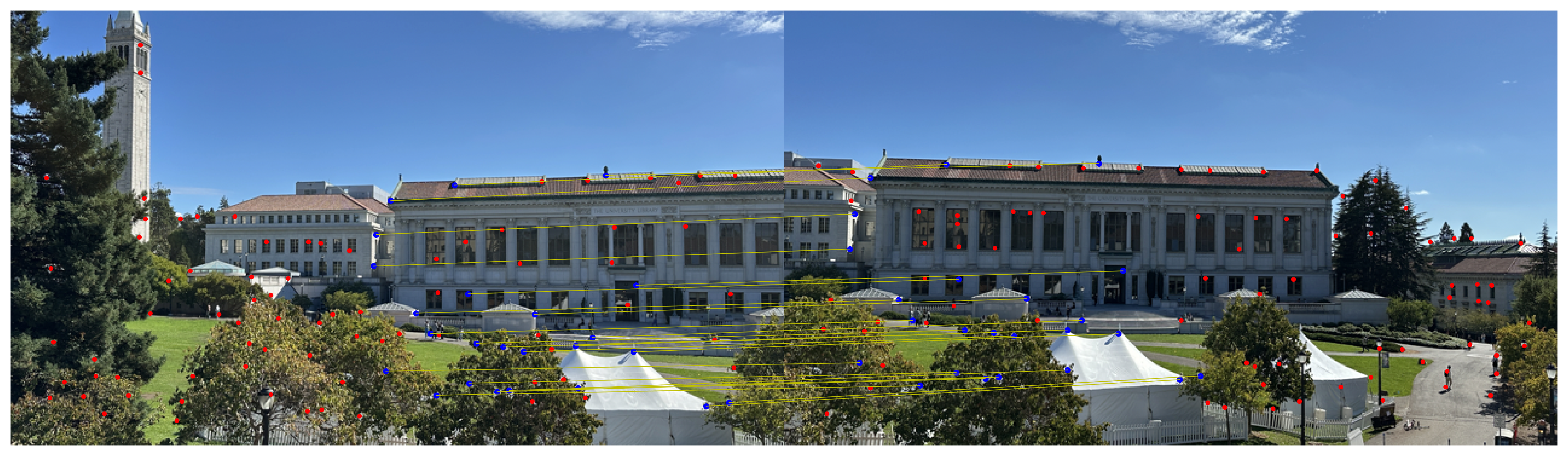
The feature matching process involves comparing feature descriptors between two images to find corresponding points. For each descriptor in the first image, the Euclidean distance to all descriptors in the second image is calculated. To filter reliable matches, Lowe’s ratio test is applied: the ratio between the distance to the nearest neighbor and the distance to the second nearest neighbor is computed, and only matches where this ratio is below a set threshold are retained. This helps eliminate ambiguous or weak matches, ensuring that the matched features are distinct and likely to correspond between the two images.
See the matching results of images below. The red point is the Harris Interest Point after ANMS and The blue point is matched points.
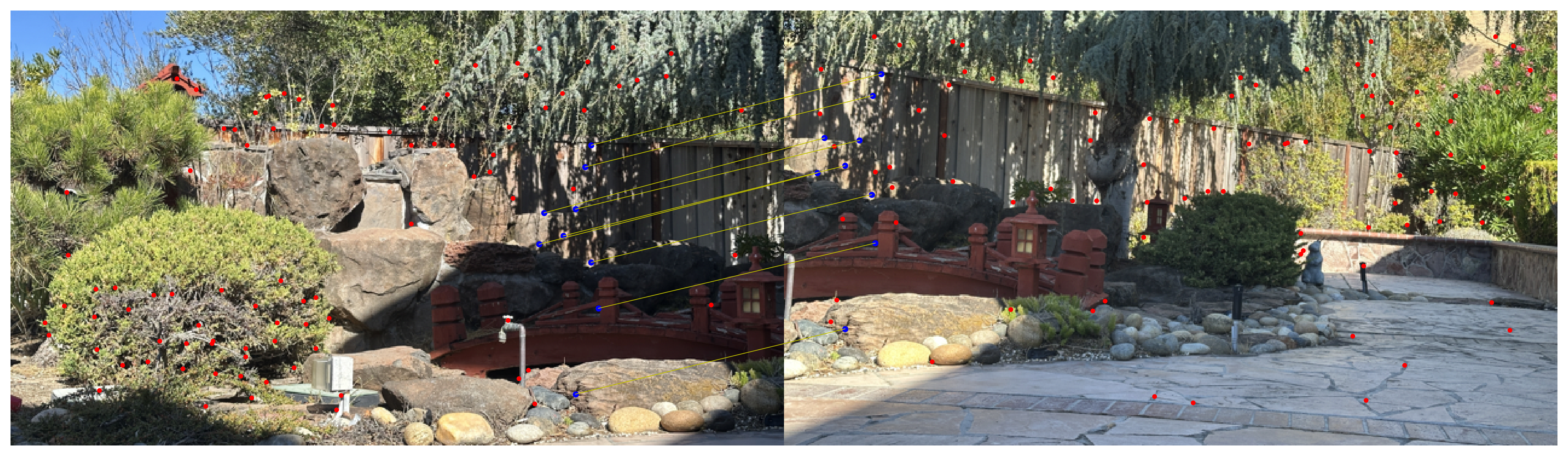
Step4: RANSAC
After selecting prominent features using Adaptive Non-Maximal Suppression (ANMS) and finding correspondences through feature matching, RANSAC (Random Sample Consensus) is applied to estimate a robust homography. The method randomly selects a minimal set of four point correspondences to compute the homography matrix, then applies the matrix to all points to identify inliers—points that fit the model within a set threshold. This process repeats for a fixed number of iterations, with the homography producing the most inliers chosen as the final estimate, effectively minimizing the impact of outliers and ensuring accurate image alignment.
Thus, we can automatically compute the homography of images and use it to stitch them together, creating a seamless mosaic.
CS180 lecture
Library
My garden
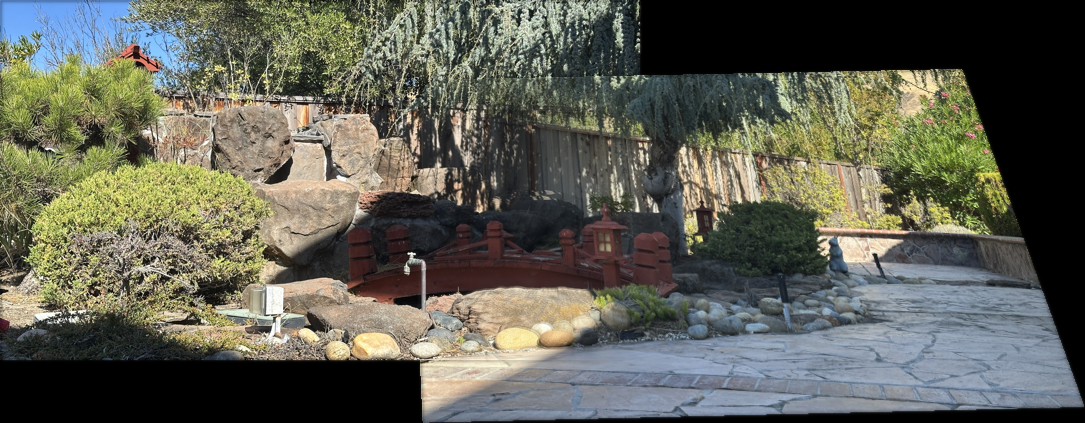
The automatic stitching achieves results comparable to manual correspondences, demonstrating the effectiveness of Harris interest points, ANMS, and the RANSAC method.
What have you learned?
Through this project, the coolest thing I have learned if the key techniques in automated image stitching, including feature detection with Harris Interest Points and refinement using ANMS for better distribution. I gained practical experience in extracting normalized feature descriptors and filtering matches using Lowe’s ratio test for reliable correspondences. Applying RANSAC highlighted the importance of robust outlier handling in estimating homography. Overall, I understood how these techniques combine to create seamless mosaics, demonstrating the effectiveness of automated approaches in image alignment and stitching tasks.